Python Quickstart

Reading and writing data files is a spatial data programmer’s bread and butter. This document explains how to use Rasterio to read existing files and to create new files. Some advanced topics are glossed over to be covered in more detail elsewhere in Rasterio’s documentation. Only the GeoTIFF format is used here, but the examples do apply to other raster data formats. It is presumed that Rasterio has been installed.

Opening a dataset in reading mode

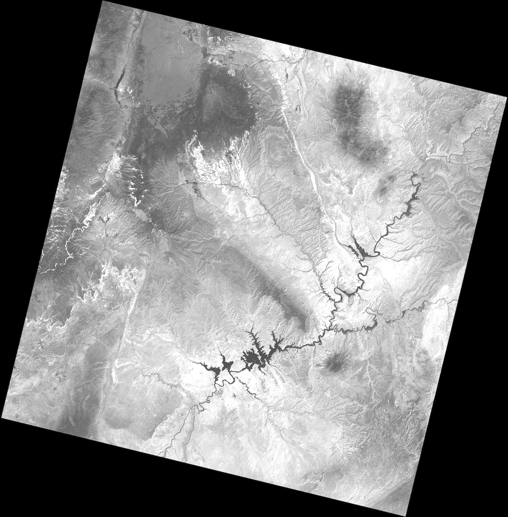
Consider a GeoTIFF file named example.tif with 16-bit Landsat 8 imagery covering a part of the United States’s Colorado Plateau [1]. Because the imagery is large (70 MB) and has a wide dynamic range it is difficult to display it in a browser. A rescaled and dynamically squashed version is shown below.

Import rasterio to begin.

>>> import rasterio

Next, open the file.

>>> dataset = rasterio.open('example.tif')

Rasterio’s open() function takes a path string or path-like object and returns an opened dataset object. The path may point to a file of any supported raster format. Rasterio will open it using the proper GDAL format driver. Dataset objects have some of the same attributes as Python file objects.

>>> dataset.name
'example.tif'
>>> dataset.mode
'r'
>>> dataset.closed
False

Dataset attributes

Properties of the raster data stored in the example GeoTIFF can be accessed through attributes of the opened dataset object. Dataset objects have bands and this example has a band count of 1.

>>> dataset.count
1

A dataset band is an array of values representing the partial distribution of a single variable in 2-dimensional (2D) space. All band arrays of a dataset have the same number of rows and columns. The variable represented by the example dataset’s sole band is Level-1 digital numbers (DN) for the Landsat 8 Operational Land Imager (OLI) band 4 (wavelengths between 640-670 nanometers). These values can be scaled to radiance or reflectance values. The array of DN values is 7731 columns wide and 7871 rows high.

>>> dataset.width
7731
>>> dataset.height
7871

Some dataset attributes expose the properties of all dataset bands via a tuple of values, one per band. To get a mapping of band indexes to variable data types, apply a dictionary comprehension to the zip() product of a dataset’s DatasetReader.indexes and DatasetReader.dtypes attributes.

>>> {i: dtype for i, dtype in zip(dataset.indexes, dataset.dtypes)}
{1: 'uint16'}

The example file’s sole band contains unsigned 16-bit integer values. The GeoTIFF format also supports signed integers and floats of different size.

Dataset georeferencing

A GIS raster dataset is different from an ordinary image; its elements (or “pixels”) are mapped to regions on the earth’s surface. Every pixels of a dataset is contained within a spatial bounding box.

>>> dataset.bounds
BoundingBox(left=358485.0, bottom=4028985.0, right=590415.0, top=4265115.0)

Our example covers the world from 358485 meters (in this case) to 590415 meters, left to right, and 4028985 meters to 4265115 meters bottom to top. It covers a region 231.93 kilometers wide by 236.13 kilometers high.

The value of DatasetReader.bounds attribute is derived from a more fundamental attribute: the dataset’s geospatial transform.

>>> dataset.transform
Affine(30.0, 0.0, 358485.0,
       0.0, -30.0, 4265115.0)

A dataset’s DatasetReader.transform is an affine transformation matrix that maps pixel locations in (col, row) coordinates to (x, y) spatial positions. The product of this matrix and (0, 0), the column and row coordinates of the upper left corner of the dataset, is the spatial position of the upper left corner.

>>> dataset.transform * (0, 0)
(358485.0, 4265115.0)

The position of the lower right corner is obtained similarly.

>>> dataset.transform * (dataset.width, dataset.height)
(590415.0, 4028985.0)

But what do these numbers mean? 4028985 meters from where? These coordinate values are relative to the origin of the dataset’s coordinate reference system (CRS).

>>> dataset.crs
CRS.from_epsg(32612)

EPSG:32612 identifies a particular coordinate reference system: UTM zone 12N. This system is used for mapping areas in the Northern Hemisphere between 108 and 114 degrees west. The upper left corner of the example dataset, (358485.0, 4265115.0), is 141.5 kilometers west of zone 12’s central meridian (111 degrees west) and 4265 kilometers north of the equator.

Between the DatasetReader.crs and DatasetReader.transform attributes, the georeferencing of a raster dataset is described and the dataset can compared to other GIS datasets.

Reading raster data

Data from a raster band can be accessed by the band’s index number. Following the GDAL convention, bands are indexed from 1.

>>> dataset.indexes
(1,)
>>> band1 = dataset.read(1)

The DatasetReader.read() method returns a numpy.ndarray.

>>> band1
array([[0, 0, 0, ..., 0, 0, 0],
       [0, 0, 0, ..., 0, 0, 0],
       [0, 0, 0, ..., 0, 0, 0],
       ...,
       [0, 0, 0, ..., 0, 0, 0],
       [0, 0, 0, ..., 0, 0, 0],
       [0, 0, 0, ..., 0, 0, 0]], dtype=uint16)

Values from the array can be addressed by their row, column index.

>>> band1[dataset.height // 2, dataset.width // 2]
17491

Spatial indexing

Datasets have an DatasetReader.index() method for getting the array indices corresponding to points in georeferenced space. To get the value for the pixel 100 kilometers east and 50 kilometers south of the dataset’s upper left corner, do the following.

>>> x, y = (dataset.bounds.left + 100000, dataset.bounds.top - 50000)
>>> row, col = dataset.index(x, y)
>>> row, col
(1666, 3333)
>>> band1[row, col]
7566

To get the spatial coordinates of a pixel, use the dataset’s DatasetReader.xy() method. The coordinates of the center of the image can be computed like this.

>>> dataset.xy(dataset.height // 2, dataset.width // 2)
(476550.0, 4149150.0)

Creating data

Reading data is only half the story. Using Rasterio dataset objects, arrays of values can be written to a raster data file and thus shared with other GIS applications such as QGIS.

As an example, consider an array of floating point values representing, e.g., a temperature or pressure anomaly field measured or modeled on a regular grid, 240 columns by 180 rows. The first and last grid points on the horizontal axis are located at 4.0 degrees west and 4.0 degrees east longitude, the first and last grid points on the vertical axis are located at 3 degrees south and 3 degrees north latitude.

>>> import numpy as np
>>> x = np.linspace(-4.0, 4.0, 240)
>>> y = np.linspace(-3.0, 3.0, 180)
>>> X, Y = np.meshgrid(x, y)
>>> Z1 = np.exp(-2 * np.log(2) * ((X - 0.5) ** 2 + (Y - 0.5) ** 2) / 1 ** 2)
>>> Z2 = np.exp(-3 * np.log(2) * ((X + 0.5) ** 2 + (Y + 0.5) ** 2) / 2.5 ** 2)
>>> Z = 10.0 * (Z2 - Z1)

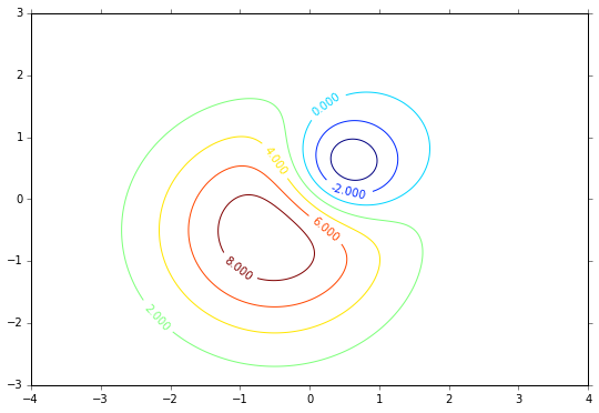
The fictional field for this example consists of the difference of two Gaussian distributions and is represented by the array Z. Its contours are shown below.

Opening a dataset in writing mode

To save this array along with georeferencing information to a new raster data file, call rasterio.open() with a path to the new file to be created, 'w' to specify writing mode, and several keyword arguments.

• driver: the name of the desired format driver

• width: the number of columns of the dataset

• height: the number of rows of the dataset

• count: a count of the dataset bands

• dtype: the data type of the dataset

• crs: a coordinate reference system identifier or description

• transform: an affine transformation matrix, and

• nodata: a “nodata” value

The first 5 of these keyword arguments parametrize fixed, format-specific properties of the data file and are required when opening a file to write. The last 3 are optional.

In this example the coordinate reference system will be '+proj=latlong', which describes an equirectangular coordinate reference system with units of decimal degrees. The proper affine transformation matrix can be computed from the matrix product of a translation and a scaling.

>>> from rasterio.transform import Affine
>>> res = (x[-1] - x[0]) / 240.0
>>> transform = Affine.translation(x[0] - res / 2, y[0] - res / 2) * Affine.scale(res, res)
>>> transform
Affine(0.033333333333333333, 0.0, -4.0166666666666666,
       0.0, 0.033333333333333333, -3.0166666666666666)

The upper left point in the example grid is at 3 degrees west and 2 degrees north. The raster pixel centered on this grid point extends res / 2, or 1/60 degrees, in each direction, hence the shift in the expression above.

A dataset for storing the example grid is opened like so

>>> new_dataset = rasterio.open(
...     '/tmp/new.tif',
...     'w',
...     driver='GTiff',
...     height=Z.shape[0],
...     width=Z.shape[1],
...     count=1,
...     dtype=Z.dtype,
...     crs='+proj=latlong',
...     transform=transform,
... )

Values for the height, width, and dtype keyword arguments are taken directly from attributes of the 2-D array, Z. Not all raster formats can support the 64-bit float values in Z, but the GeoTIFF format can.

Saving raster data

To copy the grid to the opened dataset, call the new dataset’s DatasetWriter.write() method with the grid and target band number as arguments.

>>> new_dataset.write(Z, 1)

Then call the DatasetWriter.close() method to sync data to disk and finish.

>>> new_dataset.close()

Because Rasterio’s dataset objects mimic Python’s file objects and implement Python’s context manager protocol, it is possible to do the following instead.

with rasterio.open(
    '/tmp/new.tif',
    'w',
    driver='GTiff',
    height=Z.shape[0],
    width=Z.shape[1],
    count=1,
    dtype=Z.dtype,
    crs='+proj=latlong',
    transform=transform,
) as dst:
    dst.write(Z, 1)

These are the basics of reading and writing raster data files. More features and examples are contained in the advanced topics section.

[1]

“example.tif” is an alias for band 4 of Landsat scene LC80370342016194LGN00.