Plotting

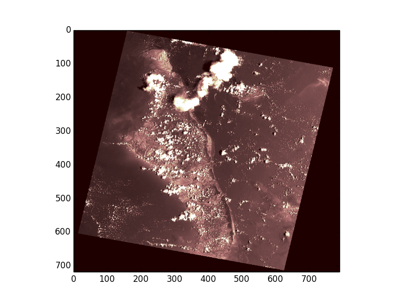
Rasterio reads raster data into numpy arrays so plotting a single band as two dimensional data can be accomplished directly with pyplot.

>>> import rasterio
>>> from matplotlib import pyplot
>>> src = rasterio.open("tests/data/RGB.byte.tif")
>>> pyplot.imshow(src.read(1), cmap='pink')
<matplotlib.image.AxesImage object at 0x...>
>>> pyplot.show()

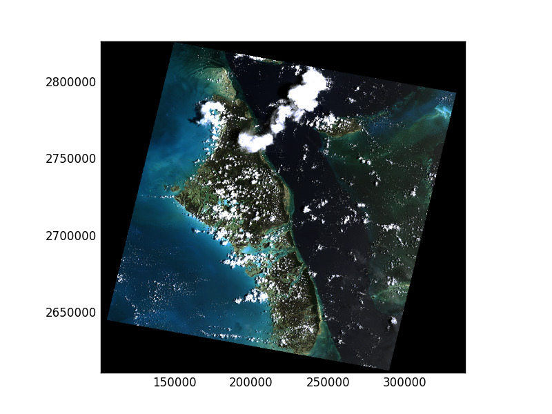
Rasterio also provides rasterio.plot.show() to perform common tasks such as displaying multi-band images as RGB and labeling the axes with proper geo-referenced extents.

The first argument to show() represent the data source to be plotted. This can be one of

• A dataset object opened in ‘r’ mode

• A single band of a source, represented by a (src, band_index) tuple

• A numpy.ndarray, 2D or 3D. If the array is 3D, ensure that it is in rasterio band order.

Thus the following operations for 3-band RGB data are equivalent. Note that when passing arrays, you can pass in a transform in order to get extent labels.

>>> from rasterio.plot import show
>>> show(src)
<matplotlib.axes._subplots.AxesSubplot object at 0x...>
>>> show(src.read(), transform=src.transform)
<matplotlib.axes._subplots.AxesSubplot object at 0x...>

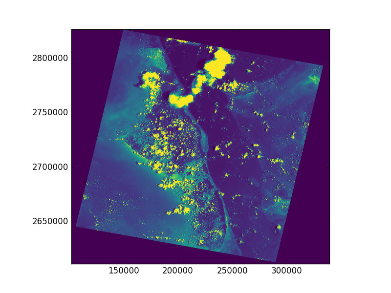
and similarly for single band plots. Note that you can pass in cmap to specify a matplotlib color ramp. Any kwargs passed to show() will be passed through to the underlying pyplot functions.

>>> show((src, 2), cmap='viridis')
<matplotlib.axes._subplots.AxesSubplot object at 0x...>
>>> show(src.read(2), transform=src.transform, cmap='viridis')
<matplotlib.axes._subplots.AxesSubplot object at 0x...>

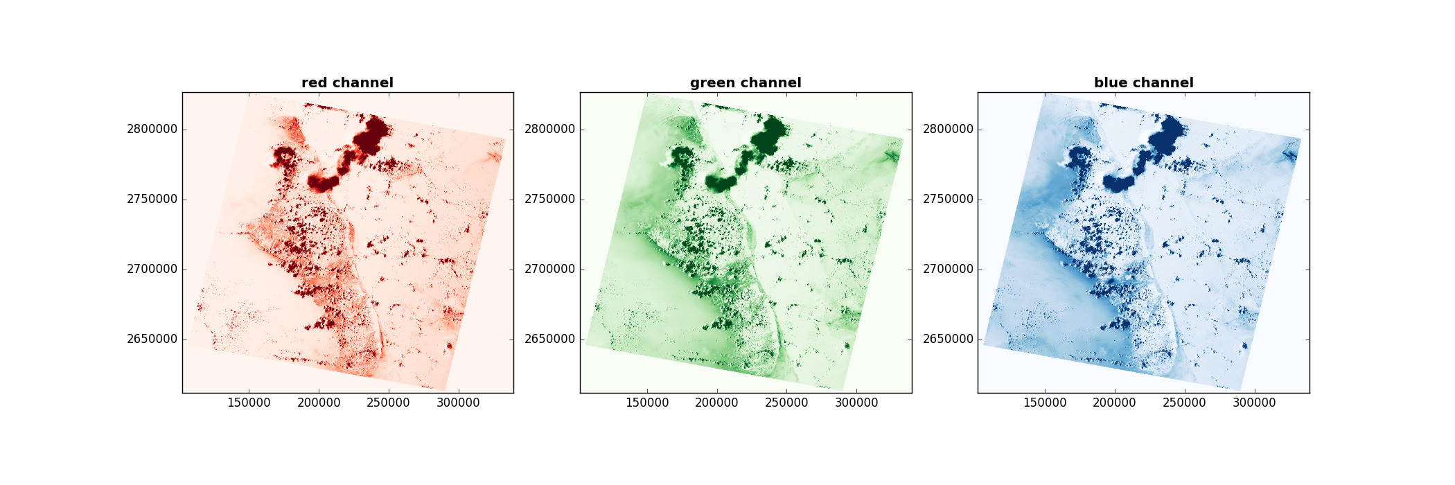
You can create a figure with multiple subplots by passing the show(..., ax=ax1) argument. Also note that this example demonstrates setting the overall figure size and sets a title for each subplot.

>>> fig, (axr, axg, axb) = pyplot.subplots(1,3, figsize=(21,7))
>>> show((src, 1), ax=axr, cmap='Reds', title='red channel')
<matplotlib.axes._subplots.AxesSubplot object at 0x...>
>>> show((src, 2), ax=axg, cmap='Greens', title='green channel')
<matplotlib.axes._subplots.AxesSubplot object at 0x...>
>>> show((src, 3), ax=axb, cmap='Blues', title='blue channel')
<matplotlib.axes._subplots.AxesSubplot object at 0x...>
>>> pyplot.show()

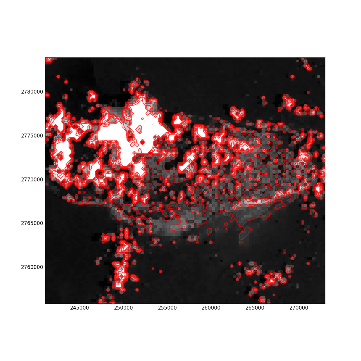
For single-band rasters, there is also an option to generate contours.

>>> fig, ax = pyplot.subplots(1, figsize=(12, 12))
>>> show((src, 1), cmap='Greys_r', interpolation='none', ax=ax)
<matplotlib.axes._subplots.AxesSubplot object at 0x...>
>>> show((src, 1), contour=True, ax=ax)
<matplotlib.axes._subplots.AxesSubplot object at 0x...>
>>> pyplot.show()

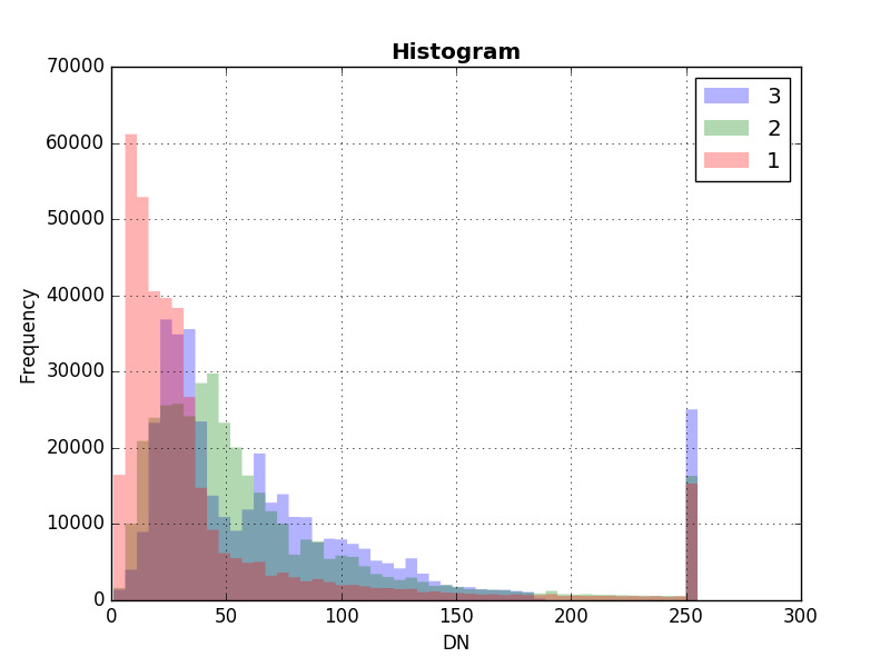
Rasterio also provides a show_hist() function for generating histograms of single or multiband rasters:

>>> from rasterio.plot import show_hist
>>> show_hist(
...     src, bins=50, lw=0.0, stacked=False, alpha=0.3,
...     histtype='stepfilled', title="Histogram")

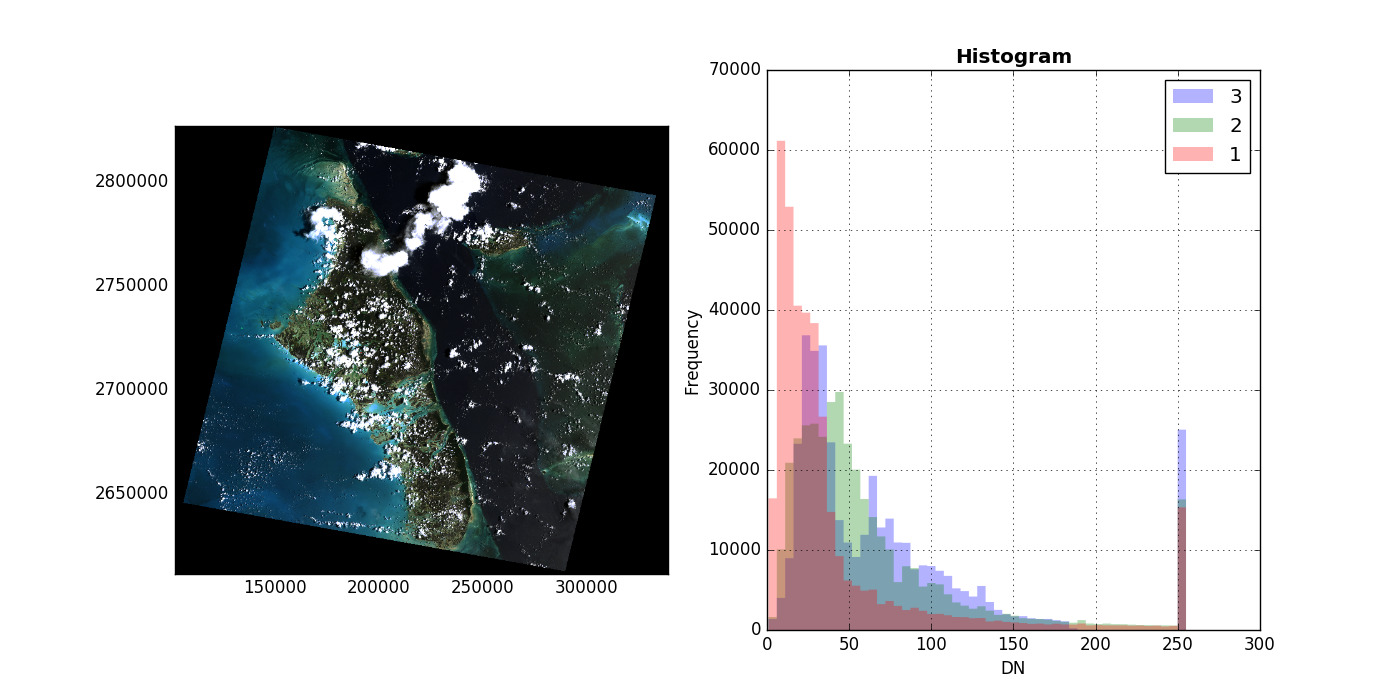
The show_hist() function also takes an ax argument to allow subplot configurations

>>> fig, (axrgb, axhist) = pyplot.subplots(1, 2, figsize=(14,7))
>>> show(src, ax=axrgb)
<matplotlib.axes._subplots.AxesSubplot object at 0x...>
>>> show_hist(src, bins=50, histtype='stepfilled',
...           lw=0.0, stacked=False, alpha=0.3, ax=axhist)
>>> pyplot.show()